Thursday 1 October 2015

Chord diagrams: when there’s too many categories to Venn!

At the moment I’m comparing differentially-expressed genes from six different transcriptome studies. With this many categories, graphically representing cross-study commonalities is challenging. Chord diagrams are visually appealing, and provide several advantages over the tradition Venn:

Venn diagrams 
  • Gene lists are represented as shapes
  • List representation is not proportional to list size (although Eulerian circles can do this)
  • Common elements (shared gene findings) are shown by shape intersection
Chord diagrams
  • Gene lists are represented as annulus segments (with larger segments indicating more implicated genes)
  • Common elements (shared gene findings) are represented by the lines connecting two segments
  • This allows emphasis of important commonalities (e.g. lines are shown in colour when two gene lists contain statistically significant overlap)

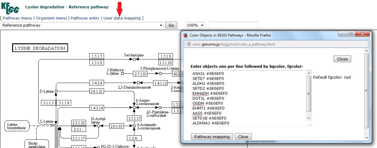
Creating a Chord diagram

Using NetworkAnalyst you can create a Chord diagram within a few minutes.
  1. Choose the ‘starting with gene or protein lists’ module
  2. Upload your gene lists
  3. Choose ‘chord diagrams’
  4. Save the image as an .svg so you can edit it in Illustrator (or freeware vector editing software)
Sometimes the .svg saved from NetworkAnalyst will crash Illustrator. If this happens, open the svg in notepad and delete the extraneous text between ‘<style type=’ and ‘</style>’. When you then open the svg in Illustrator, the lines of the cord diagram may also have fill (making the centre a solid colour). If this happens set the fill to null for all lines in the middle of the cord diagram.
  1. Click somewhere in the middle of the cord diagram
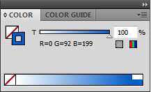
  2. From the top menu, choose ‘select/same/fill colour’. This should select everything in the centre of the diagram, and leave the annulus and text unselected
  3. In the colour window, change the fill colour to null (leaving only a stoke colour). For help using the colour tool see my earlier post
  4. Add the finishing touches to the diagram (labels, colour scheme etc)


Wednesday 30 September 2015

15th International Myopia Conference


I recently got back from the 15th International Myopia Conference in Wenzhou, China. Dr. Jia Qu did a great job organising speakers (and some interesting local food- I got my first taste of cuttlefish)! I particularly liked the ON-OFF visual pathways session where Machelle Pardue and colleagues discussed their knockout models.

The poster sessions were also great- so many proteome and transcriptome studies! I presented a time-series analysis of my electroretinogram and RNAseq data from the chick myopia model. Here’s my poster (or click here for a hi-res version).


Sunday 12 July 2015

Creating figures to depict enriched KEGG pathways: A first attempt

Gene set enrichment analysis (GSEA) of my microarray dataset implicated a number of KEGG pathways. I’m now exploring ways to create figures summarising the findings. In my last post I described mapping the core implicated genes (leading edge subset) from the analysis onto KEGG pathway diagrams. Although useful when interpreting the data, these figures are difficult to take in at a glance. In the figure below I’ve attempted to provide a stylized adaptation of the KEGG pathways to convey that many of the leading edge genes are involved in acetyl-CoA production feeding into the citrate cycle. It’s still not quite right, but getting there!


Wednesday 1 July 2015

Mapping a gene list onto KEGG pathways

In a previous post I discussed using GSEA to identify enriched KEGG pathways in my microarray data-set. After running the GSEA leading edge analysis I had a list of the genes that contributed most to the enrichment score for each pathway. I then wanted to examine where these genes fell within the KEGG pathway. The ‘user data mapping’ function in KEGG Mapper is a nice tool to achieve this quickly.

User data mapping

Select the ‘user data mapping’ option when viewing the reference KEGG pathway. In the pop-up window enter the gene symbols followed by the background and foreground color in hexadecimal numbers (if no color is specified the default is red).

Clicking ‘pathway mapping’ updates the reference to highlight the entered gene list. In this case it appears that my leading edge includes a sub-set of genes involved in methylation of histone lysine residues (in addition to the main pathway functions).

Tuesday 30 June 2015

Creating transparent fills for Igor Pro graphs

For several of my experiments I’ve profiled retinal functioning using electroretinograms (ERGs) and graphed the averages with dynamic error bars in Igor Pro. Using a transparent fill for the error bars of these graphs allows clear visualization of overlaps. Unfortunately this capability isn’t available in Igor. Exporting the graphs or layouts in EPS format and editing in Adobe Illustrator (or freeware vector editing software) provides an easy workaround.

Creating transparent error bar fills in Illustrator

  1. Open your EPS layout file in Adobe illustrator.
  2. Ungroup the objects.
    • Using the selection tool (top arrow in the left sidebar), select the entire graph/s
    • From the top menu, choose ‘object/ungroup’
  3. If you click on one of the error bar fills, you’ll notice that Igor has exported it in chunks. Grouping these chunks into a single object makes them easier to edit.
    • From the top menu, choose ‘window/pathfinder’ (this will open the pathfinder window).
    • Select a chunk of fill from one of the waves using the selection tool.
    • From the top menu, choose ‘select/same/fill color’.
    • Click on the first shape mode (unite) in the pathfinder window. The error bars of this color are now a single object.
  4. Edit the opacity value of the error bars.
    • With the error bars still selected, edit the opacity value in the transparency window (if you don’t have this window in your right sidebar, select ‘window/transparency’). In the example above I’ve set the opacity to 55% for all of the wave errors.
  5. When you deselect the object you’ll notice that there are some outlines remaining. These are darker as they overlap with the underlying fill.
    • Click on one of the lines. From the top menu choose, ‘select/same/stroke colour’. Hit delete to remove the extraneous lines.
  6. Repeat these steps for each of your fill colors. Once you’ve finished you can tweak the graph colors as necessary using the color and transparency palettes (see below for tips on using global color swatches to do this). 

Creating a global swatch to quickly edit a color across your entire layout

If you update the color of a global swatch, all objects using that swatch are also updated. This means that you can edit a color across the entire layout simultaneously. You can also save your swatch library for future use.

Creating a global swatch

Select a line (e.g. the wave average) from one graph. In the color window you’ll notice that there are two boxes- one indicates the stroke color and the other the fill color. Because you’ve selected a line (rather than a fill), the fill color is blank. 
Click on the stroke color box to bring it to the foreground.

In the swatch window, click ‘new swatch’.
In the popup window, tick ‘global’ and click ‘okay’. Your new swatch should now appear in the swatch window. You can double-click on it to open the swatch options menu and edit the color.

Apply the global swatch to all of the relevant fill/stroke colors in the layout

  1. Using the selection tool, select the fill or stroke color you want to change. 
  2. In the top menu, choose ‘select/same/fill color’ (or stroke color).
  3. Make sure the appropriate fill or stroke box is in the foreground in the swatch window.
  4. Click on the global swatch color you want to apply. This will apply the color across the selected objects in your layout.

Friday 19 June 2015

Brewer colour palettes for data visualization

I recently attended talk on data visualization by Martin Krzywinski hosted by VLSCI. Martin provided some great tips for presenting bioinformatics data (for some beautiful examples see Martin’s website).

At the time I was trying to categorize lists of differentially-expressed genes into Gene Ontologies (GO) using PANTHER and visualize them in a pie chart. Choosing an effective color palette to represent the 12 GO categories wasn't easy!

Martin recommended Brewer Palates, created by cartographer Cynthia Brewer. These palettes provide color scales for qualitative, quantitative, and diverging variables. The colorbrewer website is easy to use: simply choose the number of data classes and the nature of the data (qualitative, quantitative, or diverging). The resulting color scheme is provided in HEX, RGB, or CMYK, with an option to directly export a swatch into Photoshop or Illustrator. You can exclude options that aren’t color-blind, print, or photocopy safe (although not for 12 categories).


I was creating the pie charts in excel, so I entered the RGB values directly in chart tools. I now use this chart template all the time.


Tuesday 2 June 2015

Analyzing pathway expression using GSEA

For my first study I profiled gene expression in the retina/RPE/choroid using microarray and analyzed the resulting data-sets using Gene Set Enrichment Analysis (GSEA). GSEA evaluates genome-wide expression profiles to determine whether classes of genes (gene sets) are over-represented. These gene sets are based on a priori knowledge, such as KEGG pathways. GSEAs strength lies in its ability to identify subtle changes distributed across a transcript network that may be missed by more traditional single-gene analyses approaches. This approach can unify results across seemingly disparate related data-sets, which is valuable in a research area like mine where relatively few similarities have been identified across the transcriptome-wide studies conducted to date. On a practical level, the results of GSEA are also more interpretable than large lists of individual differentially-expressed genes as they are based in an established biological framework.

When I first started using GSEA to evaluate my dataset our lab had a subscription to Pathway Studio. The Pathway Studio implementation was easy to use and had great graphics; unfortunately our licence expired before I was finished. I switched to the Broad Institute’s GSEA software using the graphical java interface. I’m now glad I was forced to move to a freeware platform, as I think the Broad software gave me greater control of the analysis and the ability to explore the results in more depth. 

The Broad GSEA wiki provides a useful over-view of how to use the application. I found that leading edge analysis was a particularly important tool when interpreting results. This analysis identifies the core genes responsible for enrichment of a gene set, and over-lap in these genes across enriched pathways.

Thursday 14 May 2015

ARVO 2015: My first international conference!


This year’s ARVO conference was in Denver, Colorado. I was very excited; I’d never been to the States, or to a big conference. It was great, but I wish I had more time to see everything! I presented RNAseq GSEA data showing that structural and metabolic pathways are correlated with the eye size during myopia and hyperopia induction in chicks. Here’s my obligatory awkward first conference poster pic (and a great snap I took of the view near Estes Park, a few hours’ drive from Denver). For a better look at my poster click here.


Friday 1 May 2015

Welcome

I’m a PhD candidate at La Trobe University in Melbourne. I completed my undergrad degree in Psychological Science, and I’m now delving into the exciting world of biology and ‘omic data’. My research focuses on investigating the biological mechanisms underlying ocular growth control and the development of myopia (short-sightedness). With my submission date (almost) in sight, I’ve started this blog to chronicle my successes and failures as I explore ways to analyse, interpret, and display my data.

For more about my research, check out ResearchGate or click on the publication links below.


Publications
Murphy, M., Riddell, N., Crewther, D.P., Simpson, D., & Crewther, S.G. (2018). Temporal whole field sawtooth flicker without a spatial component elicits a myopic shift following optical defocus irrespective of waveform direction in chicks. PeerJ, 7, e6277.

Giummarra, L., Crewther, S.G., Riddell, N., Murphy, M., & Crewther, D.P. (2018). Pathway analysis identifies altered mitochondrial metabolism, neurotransmission, structural pathways and complement cascade in retina/RPE/choroid in chick model of form-deprivation myopia. PeerJ, 6, e5048.

Riddell, N., Faou, P., Crewther, S.G. (2018). Short term optical defocus perturbs normal developmental shifts in retina/RPE protein abundance. BMC Developmental Biology, 18, 18.

Riddell, N., Faou, P., Murphy, M., Giummarra, L., Downs, R., & Crewther, S.G. (2017). The retina/RPE proteome in chick myopia and hyperopia models: commonalities with inherited and age-related ocular pathologies. Molecular Vision, 23, 872-888.

Riddell, N., & Crewther, S. G. (2017). Novel evidence for complement system activation in chick myopia and hyperopia models: a meta-analysis of transcriptome datasets. Scientific Reports, 7, 9719.

Riddell, N., & Crewther, S. G. (2017). Integrated comparison of GWAS, transcriptome, and proteomics studies highlights similarities in the biological basis of animal and human myopia. Investigative Ophthalmology & Visual Science, 58(1), 660-669.

Riddell, N., Giummarra, L., Hall, N. E., & Crewther, S. G. (2016). Bidirectional expression of metabolic, structural, and immune pathways in early myopia and hyperopia. Frontiers in Neuroscience, 10.

Riddell, N., Hugrass, L., Jayasuriya, J., Crewther, S. G., & Crewther, D. P. (2016). An asymmetric outer retinal response to drifting sawtooth gratings. Journal of Neurophysiology, 115(5), 2349-2358.